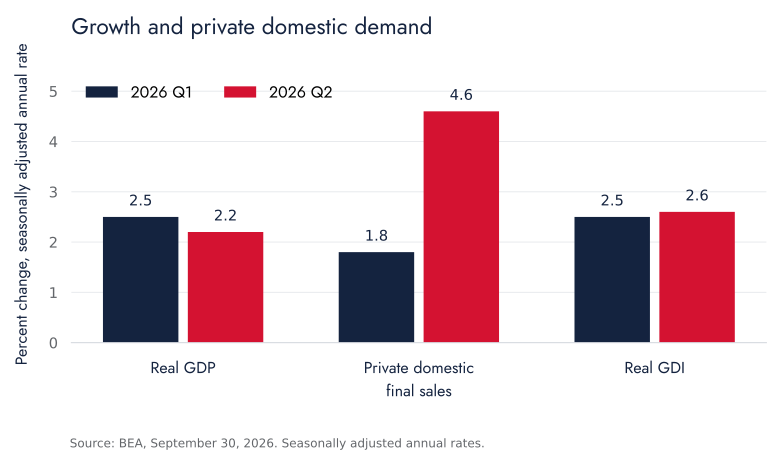
The second-quarter U.S. national accounts describe stronger private domestic demand than the headline GDP rate alone suggests. In the September 30, 2026 vintage, real GDP growth slowed from the first quarter while real final sales to private domestic purchasers accelerated. The distinction changes the question for business planning: which purchases are expanding, how much domestic production they support, and what could sustain them.
It does not establish that every household, industry, or region experienced an improvement. Aggregate spending describes a total across different purchasers and products. Assessing its durability requires evidence about income, financing, investment composition, and the connection between expenditure and production.
A divergence within the expenditure accounts
BEA's third estimate for the second quarter of 2026 reports the following measures. Both quarters in this table use that release vintage, including its annual revisions.
| Real measure |
First quarter 2026 |
Second quarter 2026 |
| GDP |
2.5% |
2.2% |
| Final sales to private domestic purchasers |
1.8% |
4.6% |
| Gross domestic income |
2.5% |
2.6% |
Rates are seasonally adjusted annual rates of change from the preceding quarter. The table does not show year-over-year growth. Final sales to private domestic purchasers combines consumer spending and gross private fixed investment. BEA identifies consumption, investment, and exports as contributors to second-quarter GDP growth, while imports also increased.
The analytical implication is narrower than a broad claim of accelerating economic activity. A measure focused on private final purchases strengthened even as the measured pace of domestic production eased. To explain the difference, the analysis must examine the expenditure categories outside that private-purchases aggregate and the domestic production embodied in purchases. It cannot assign the gap to one category simply by subtracting the two growth rates.
This separation is useful because corporate revenue opportunities are often closer to particular expenditures than to aggregate GDP. A seller of business equipment, a residential builder, and a consumer-services provider do not face the same demand composition. A common macroeconomic headline is a starting point for those markets, not a substitute for examining them.
Consumption covers more than discretionary retail demand
Personal consumption expenditures is broader than purchases made at retail stores. BEA's PCE methodology covers goods and services consumed by resident households and nonprofit institutions serving households. It includes expenditures made on their behalf and imputations, including owner-occupied housing services.
Consequently, the strength of aggregate consumption need not translate proportionately into cash spending on discretionary goods. A shift toward medical care, housing services, or another large category changes the connection between the aggregate and a particular business. The appropriate commercial question identifies the relevant category, the price adjustment, and the purchaser rather than treating total PCE as one homogeneous market.
Income provides an essential counterpart. The August 2026 income and outlays release, also published September 30, reports a 0.6 percent monthly increase in real PCE and no change in real disposable personal income. It places the personal saving rate at 4.1 percent. These are monthly observations and are not directly comparable with annualized quarterly rates.
That single month does not establish an unsustainable consumption path. It does identify questions that a durability assessment should investigate: whether spending is supported by persistent income growth, changes in saving, borrowing, or a temporary timing effect. A national saving rate is not an estimate of the cash buffer available to each household.
An aggregate can also conceal different marginal responses. Households facing a high required payment may adjust spending differently from households with substantial liquid assets. An assertion about which group is driving consumption requires distributional evidence. The aggregate income and spending releases cited here cannot establish that attribution by themselves.
Fixed investment combines different demand channels
BEA's private fixed investment methodology includes structures, equipment, and intellectual property products, as well as residential investment. It covers additions, improvements, and replacement of assets. Investment in this national-accounts sense is distinct from acquiring a financial security.
These components differ in timing and economic role. Construction can generate expenditure over an extended period. Equipment can be purchased domestically or imported. Intellectual property can involve purchased products or production for an enterprise's own use. Housing investment responds to conditions different from those governing a company's computing investment or factory expansion.
A rise in fixed investment therefore requires a second decomposition before it is interpreted as broad business confidence or a uniform expansion of productive capacity. Replacement can maintain an existing capability. A project can increase capacity only after complementary equipment, workers, connections, and operating arrangements are available. The expenditure flow and the resulting service flow are related but distinct.
For planning, the relevant evidence includes the type of asset, stage of delivery, expected use, financing terms, and exposure to imported inputs. A firm supplying installation services may benefit at a different point from the firm that will eventually operate the asset. A forecast based on the aggregate alone can miss those differences even when its national growth assumption is correct.
Domestic purchases and domestic production
As described in BEA's net-exports methodology, an import can be part of a purchase by a U.S. resident without representing U.S. production. National accounts must remove the imported content included in expenditure measures when measuring domestic output. This accounting treatment does not establish that the import harmed productive capacity or that it can be eliminated without changing the associated purchase.
Consider a hypothetical company buying equipment for 100 monetary units, of which 70 represents imported equipment and 30 represents services produced domestically. In this deliberately simplified illustration, fixed investment records 100 and imports record 70, leaving 30 in domestic expenditure-side GDP from these transactions. There are no inventories, taxes, or other transactions in the example.
The accounting explains how strong equipment purchases can coincide with a smaller immediate contribution to domestic production. It does not measure the equipment's future services, productivity effect, or the domestic value added generated by operating it. Those are subsequent outcomes requiring evidence about utilization and production.
This also limits the interpretation of a negative import contribution in a growth release. The contribution is part of an accounting decomposition. It is not an estimate of the GDP gain available from preventing the imports while leaving every other expenditure unchanged. Such a counterfactual requires a model of substitution, prices, capacity, and demand.
Inventories require a separate reading
Final sales excludes inventory investment, while GDP includes it. BEA's inventory methodology defines inventory investment as additions less withdrawals from stocks in physical-volume terms. Inventory investment concerns the change in stocks, and its contribution to growth depends on how that flow changes. Businesses can continue accumulating inventories at a slower pace while inventories subtract from GDP growth.
An original hypothetical example illustrates the distinction. Suppose stocks rise by 20 in one quarter and by 10 in the next, with no price changes or other complications. Inventories are still increasing in the second quarter, but the flow of inventory investment has fallen by 10. Describing that change as firms necessarily running down their stocks would confuse a slower accumulation with an actual decline in the stock.
The business interpretation requires further information. Inventories can increase because firms expect sales, because delivery conditions improve, or because sales fall short of expectations. The same stock movement can therefore signal different operating conditions. Orders, shipments, sales, delivery times, and the composition of inventories help distinguish those explanations.
This study does not estimate the inventory contribution to second-quarter growth. Its purpose is to identify why a demand assessment should not infer inventory behavior from the gap between two headline rates without the appropriate contribution data.
A disciplined assessment of durability
The available evidence supports examining private demand separately from the GDP headline. It does not support a forecast based solely on repeating one quarter's rate. A more complete assessment would bring together real income and consumption categories, fixed-investment components, financing conditions, inventory flows, and the domestic content of demand.
Those inputs should be linked to explicit propositions. Consumption supported by continuing income growth presents a different prospect from spending supported by a temporary reduction in saving. Investment that expands productive services presents a different prospect from a brief surge in replacement purchases. A one-time inventory adjustment differs from sustained final demand. The evidence needed to distinguish these cases is identifiable even where the conclusion remains uncertain.
For executives, the practical output is a demand map tied to the company's customers, products, and production stage. For policy professionals, it is an assessment that separates observed expenditure from claims about productive capacity or policy effects. Both uses benefit from the same discipline: maintain consistent definitions, use a common data vintage, and specify which mechanism explains the judgment.